CPU Profiling
Understand basics of CPU profiling in 5 minutes ⏱️!
Example
This guide will demonstrate CPU profiling using go, but these fundamentals apply to any language. Let's walk through an example of CPU profiling.
Capturing data
Take the following example of a go program that has a main function, that first calls iterateLong which calls iterate with 9 billion iterations, and then iterateShort, which calls iterate with 1 billion iterations.
package main

func main() {
    iterateLong()
    iterateShort()
}

func iterateLong() {
    iterate(9_000_000_000)
}

func iterateShort() {
    iterate(1_000_000_000)
}

func iterate(iterations int) {
    for i := 0; i < iterations; i++ {
    }
}
When executed this program takes 5 seconds to execute in total (on an AMD Ryzen 5 3400GE CPU). With profiling we can understand what was executing during those 5 seconds and for how long. For the sake of simplicity, a sampling CPU profiler looks at the "current" stack trace 100x per second (the sampling rate is typically configurable, but 100x is both common and easier to calculate with).
Data format
With a profiler running during the execution of the above program it records a profile, that produces the following data in folded stack trace format:
main;iterateLong;iterate 450
main;iterateShort;iterate 50
Parca uses the open standard
pprof, which is optimized to use as little space as possible, but folded stack traces are great for human readability.
10% (50 samples observed out of 500) of the time was spent in the iterate function called by iterateShort and 90% (450 samples observed out of 500) of the time was spent in the iterate function called by iterateLong.
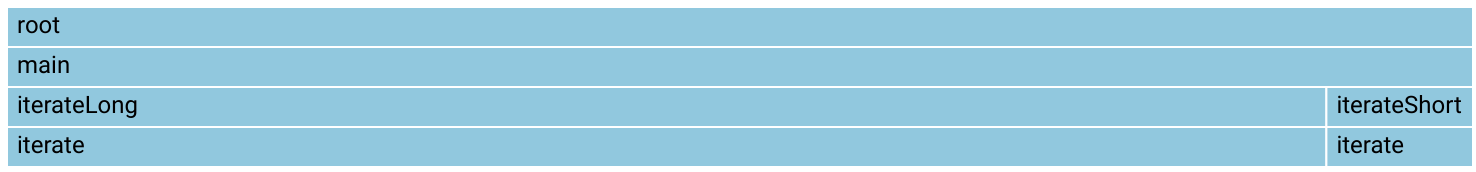
Visualizing
Using this data, a popular way to visualize profiling data is using Flame Graphs, or as they are called when they are built from the top being the root, Icicle Graphs.
Recap
In this guide you have learned the basic fundamentals of CPU profiling:
- How data is captured: by observing the executed stack traces 100x per second.
- What the raw data looks like: folded stack traces, and the optimized pprof format.
- Useful ways to visualize data: Flamegraphs/Icicle-Graphs.
Congrats! 🎉